Home >
Blog >
Proximity Study Along Rural Highways - Injurious Affection assessment
Proximity Study Along Rural Highways - Injurious Affection assessment
Posted
on 5 November 2025
Source: IRWA
A proximity study of rural residential properties along busy highways in Jefferson County, Wisconsin, was performed in February 2020∗ to assist in the valuation of the potential for severance damages to the home improvement value as a result of fee acquisitions for a road project which resulted in numerous parcels having a decreased distance to the right of way line (ROW). The Wisconsin Department of Transportation project was located along a busy state highway.
Per the county zoning, the current required minimum setback from the ROW to a residential home is 100 feet to a principle arterial highway, 70 feet to a minor arterial highway, and 50 feet to a major and minor collector highway. The setback from the centerline was greater, depending on the highway classification. The more restrictive setback applies. In all cases within this study, the setback from the ROW was more restrictive, and the distance to the ROW is the focus of this study.
Two project parcels that were conforming before the project became non-conforming after, 73 feet and 53 feet to the ROW before and 41 feet and 40 feet, respectively, after.
Four other sites were non-conforming in the before condition with distances to the existing ROW ranging from 9 feet to 47 feet and became even closer to the proposed ROW after ranging from 3 feet to 40 feet.
Three other sites became closer to the required minimum setback and ranged from 67 feet to 81 feet before to a range of 52 feet to 63 feet after. The construction years of the homes along the project ranged from around 1900 to the 1970s, with one newer home from the 1990s.
Background Analysis Techniques
The magnitude of the change in market value of a home as a function of the home’s distance to the ROW (setback) is difficult to observe in a limited data set. Interviews with real estate agents suggest that a residential property that is located notably close to the ROW can sell for 5% to 10% less as compared to a residential property located at an acceptable distance to the ROW.
One way to estimate whether there is a change in the market value of a home improvement due to a decreased setback is to derive this difference (if any) using paired sales. This involves selecting sales in the before condition for a given setback and then finding comparable sales with a decreased setback in the after condition. The paired sales are analyzed and a difference, if any, is attributed to the difference in the home’s setback to the ROW.
A paired sales analysis can be a useful tool to observe large magnitude differences, but it is difficult to find two such data sets for comparison when there is a modest difference in the distance to the ROW. Additionally, physical differences can make it difficult to derive a difference in the home improvement value due to relatively small changes in distance to the ROW. For this project, the appraiser has not attempted to perform a paired sales analysis approach to evaluate differences in home improvement value due to differing setbacks.
Selected Study Methodology
Another method of deriving a relationship between unit sale price of a home and the distance to the ROW can be made using a large set of data with homes of varying setbacks. Using sales with a wide range of setbacks and including sales of homes very close to the ROW, the appraiser evaluated whether there is a difference in market value due to a decrease in the distance to the ROW. This is a mass appraisal technique, with the expected results to be an averaged trend of the data. Distance of the home improvement versus the adjusted home improvement unit values are graphed, and a best fit line is established. Questions to be answered included:
What is an acceptable setback such that for greater setbacks, there is little further observable change in market unit value?
What is the magnitude or percent of change in unit value as the distance to the ROW becomes closer to zero in a before and after situation?
Sales Research
The sales of improved rural residential properties along busy county or state highways were researched across the county. Sites located in areas where the speed limit is less than 45 miles per hours as well as sites that are in municipal locations were excluded.
The appraiser researched sales from the Multiple Listing Service (MLS) website. Due to the lack of sales in any given year, it was necessary to go back in time to achieve a larger data set. Sales data starting from 2013 through February 2020 were researched.
For each sale, photos included MLS were reviewed, and descriptions were reviewed for indications of recent updates. Based on this information within the various groupings of construction dates, the homes’ ages/condition were rated using MLS descriptions and photos as well as the real estate condition reports. Other data researched included assessment records, land use and sanitary permits and GIS aerial mapping. For each sale, the appraiser estimated the land area net of existing ROW using the county GIS measurement tool.
Selected Sales
In summary, 56 sales were selected for the study. The sale dates ranged from July 2013 to January 2020. The homes ranged in size from 768 square feet to 2,794 square feet. The homes were built within the range of 1888 to 2007. The sites had various garages and outbuildings.
The land areas net of existing ROW ranged from 0.4 to 26.35 acres, with most in the range of one acre to about 4 acres. The two sales with large land areas were later excluded, resulting in a range of 0.4 acres to 4.35 acres.
Distance to ROW ranged from 0.1 feet to 346 feet. Homes with setbacks greater than 180 feet were normalized to 180 feet. This was performed for three sales. Since the setback distance of interest is much less than 180 feet, this adjustment does not affect the graph.
Considering the entire data set, the unadjusted sale prices ranged from $108,500 to $340,000 with an average of $231,295 and a median of $234,310. The unadjusted price per square foot (SF) ranged from $50.77 to $212.24, with an average of $133.04 per SF and a median of $124.37 per SF. Three sales were excluded and the resulting range for further inclusion in the study ranged from $73.67 to $212.24 per SF.
Entire Data Set
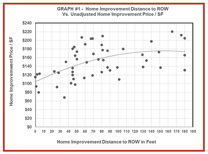
The factual data was tabulated. Prior to any adjustments, the raw data was graphed (Graph #1) using the distance to the ROW of the home improvement versus the overall sale price divided by the home’s square footage to indicate the unit sale price per SF. Based on Graph #1, a best fit line was developed. The graph indicates there is an apparent decreasing price per SF for shorter setbacks. This is encouraging data, so further analysis was performed.
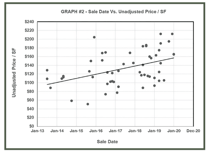
Graph #2 was prepared using sale date versus unit sale price per home square footage. This data clearly indicates an increasing upward trend in sale prices though time, as expected.
Direct Adjustments
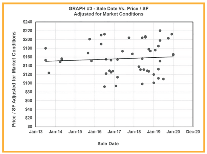
After the concluded adjustments for market conditions were made, the unadjusted sales were graphed and compared against the market adjusted sales. February 2020 was used as the appraisal date. Two very low unit prices and one very high unit price are excluded as they are clearly outliers that skewed the data.
The resulting Graph #3 of sale date versus market adjusted unit prices indicates a nearly level average price, which is expected if the data is adjusted appropriately for market conditions. The data has been normalized to reflect February 2020 prices.
Following these basic adjustments, the appraiser graphed the distance to the ROW against the unit sale prices based on the square footage of each home that sold. Outliers were identified and evaluated for reasonableness. Of the initial sales, at this point, a total of seven sales were excluded. The cost of immediate repairs was added to the sale price.
Deduct Land Value to Isolate Improvement Value
In order to derive the value of the improvements only, the next step in the process was to deduct the land value from the sale price. The land values were estimated based on the sales study for rural residential land sales previously performed as of February 2020.
Summary of Initial Findings — Entire Data Set
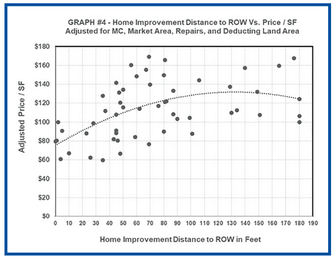
Following this round of direct adjustments, Graph #4 depicts the unit sale price per SF was graphed as a function of the home improvement distance to the ROW. Based on Graph #4, there is an apparent difference in the unit value of the improvements as a function of the home building area.
Comparative Adjustments — Entire Data Set
Based on the above analysis, the appraiser performed additional comparative adjustments to isolate the home improvement unit value. The improvements include more than just the home; rather, they include attached and detached residential garages, outbuildings, well and septic, site improvements and landscaping. The details of these adjustments are based on the market for the various ages of the buildings. Adjustments for landscaping are made by reviewing aerial photographs on the county GIS and photographs on MLS.
Comparative Analysis — Three Construction Date Ranges
Based on the entire data set, the appraiser is of the opinion that adjustments for age and condition and size would be too difficult using such a wide range of ages. The sales data was separated into three year-built groups for further analysis. The concluded construction dates were grouped as follows:
1900 or earlier to 1945
1947 to 1974
1983 to 2007
There are no sales of properties with home construction dates in 1946 or between 1975 and 1982.
For the results to be meaningful, the data was adjusted to be comparable to a theoretical average home within each of the date ranges (1900 to 1945, 1947 to 1974, and 1983 to 2007). This approach is a normalization of the data, so that the final graph includes homes that have been adjusted to have the same square footage, the same quality and condition, and the same number of bathrooms and bedrooms.
Sales with Construction Dates of 1900 to 1945
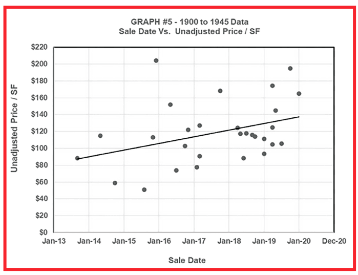
For the 1900 to 1945 data, Graph #5 depicts the unadjusted data was graphed for sale date versus unadjusted home improvement value per SF. Of note is that one sale with a setback of 226.31 feet was assigned a setback at the upper end of the remaining sales, at 150 feet. Because the setbacks of this magnitude are not considered to be affected by this setback, this had no effect on the graph, except for shortening the x-axis for better visualization of most of the data.
The best fit line increases through time, as is expected. After adjustments are made for market conditions, the resulting best fit linear trendline is nearly level, indicating satisfactory adjustments were made for market conditions.
For the 1900 to 1945 data, adjustments were made to reflect an average quality/condition of the theoretical average. This parameter required several iterations. The goal was to adjust for the fewest number of sales. The appraiser was surprised at the number of homes that were in move-in condition, and this became the average of the data.
Adjustments were also made for other significant features or lack thereof, home size, bedrooms and bathrooms as compared to the concluded average home to achieve a normalized SF comparison.
It is important to note that the goal is not to derive a single data point average for a given setback, as this is deemed not possible. Rather, the data will have a range of per SF prices for a given setback. The average of the data is concluded to be appropriate for the purposes of this analysis.
Conclusions — 1900 to 1945 Data
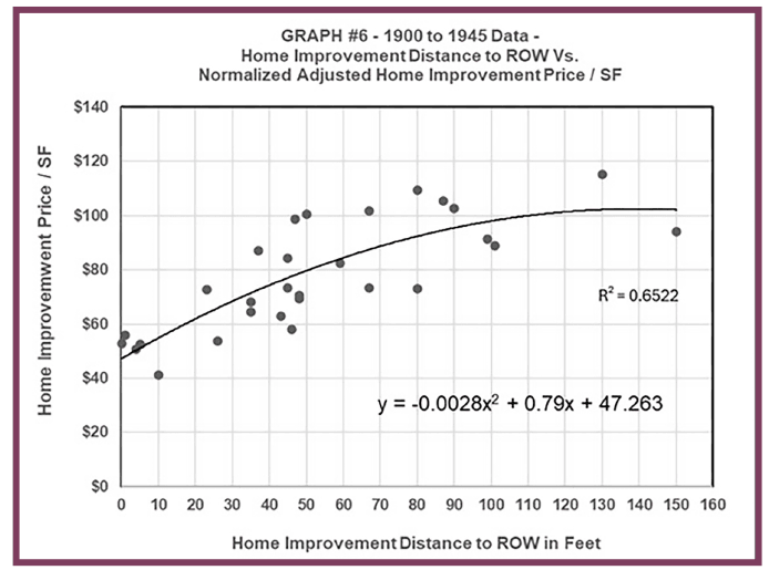
The data set was graphed following the above adjustments and a best fit polynomial regression line and equation are displayed on Graph #6. R-squared is a statistical measure that represents the proportion of the variance for a dependent variable (y) explained by an independent variable (x) in a regression model. R-squared is valid for linear regression models that use polynomials to model curvature. The R-squared value on Graph #6 is 65%, which is acceptable, and is at the low end of a strong correlation.
Based on the data as indicated on Graph #6 there is a notable decrease in price per SF for setbacks less than 35 feet. At 45 feet, there is a wide range of data. With the exception of one low data point, the data for setbacks greater than 50 feet fall above the midpoint of the data at 45 feet.
At an acceptable setback, there is theoretically no difference in the unit value, which is expected. Based on the adjusted data set, there is a definite breakpoint at about 45 feet. The results indicate no significant difference with increasing setbacks greater than about 50 feet.
Based on the 1900 to 1945 data and subject parcels with homes constructed within this date range, the appraiser relied upon Graph #6 for subject parcel setbacks that range from less than 50 feet before the project to less than 50 feet after the project.
Sales with Construction Dates of 1947 to 1974
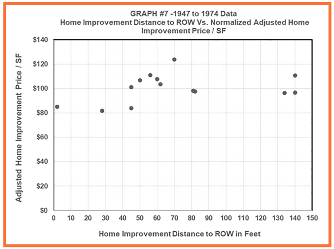
The graph of the unadjusted data for the 1947 to 1974 data was also made. Of note is that two sales had high setbacks and are assigned a setback at the upper end of the remaining sales, at 140 feet. Because the setbacks of this magnitude are not considered, this had no effect on the graph, except for shortening the x-axis for better visualization of most of the data.
The unadjusted data was also graphed through time and indicates increasing unit prices, as expected. Due to the lower number of data points, adjustments for market conditions do not appear as appropriate as expected. However, the three lowest data points occurred during 2016, and these homes have the lowest three setbacks. The appraiser concludes the adjustment for market conditions is appropriate considering the data.
The sequence and type of adjustments, as appropriate for this data set, were the same as for the 1900 to 1945 data
Conclusions — 1947 to 1974 Data
Based on the data, Graph #7 indicates a breakpoint in the data around 45 feet. Data points for setbacks greater than about 45 feet are fairly level. At an acceptable setback, there is theoretically no difference in the unit value, which is expected. However, because there are so few data points less than 50 feet, the data is of limited use.
Sales with Construction Dates of 1983 to 2007
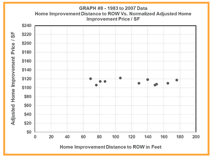
For the 1983 to 2007 sales data, the unadjusted graph indicates no trend or difference in market value based on distance to the ROW. However, no home in this data range has a distance less than 69 feet to the ROW. Through time, zoning ordinances have changed setback requirements. When homes were constructed in the early to mid-1900s, no setback requirements were in place.
Conclusions — 1983 to 2007 Data
Even after the appraiser adjusted for market conditions, Graph #8 indicates there is no apparent difference in price per SF for the data presented. The appraiser concludes there is no difference in market unit value of the home improvements for distances greater than 69 feet to the ROW for homes constructed between 1983 and 2007.
Summary and Conclusions
Sales data for homes constructed along busy highways in Jefferson County is adjusted to be comparable to a theoretical average home for three construction data ranges. As the data for each sale in a given age range is being adjusted to the same characteristics of one average theoretical home, the physical data is comparable except for the setback distance to the roadway. This method is a mass appraisal technique and a single unit value at each setback distance is not expected. Variations in the data are a result of other home features that are not adjusted for. The range in the data is concluded to be acceptable, and the results are believed to be statistically significant as presented.
The adjusted home improvement unit price for each sale is graphed against the distance to the ROW, and a best fit line is drawn using Excel. Using the setback distances for each data set, the relationship is polynomial in that as the distance to the ROW decreases, and approaches zero, the home’s improvement unit value decreases more rapidly. By comparison, as the distance to the ROW increases, the slope of the graph flattens out. This indicates that at an acceptable distance to the ROW, there is essentially no change in the market unit value as the distance increases from that point. The resulting graph shows the data points falling closer to the best fit trend line as compared to the unadjusted data, which is expected.
Based on the appraiser’s research, for rural residential properties located on busy highways, the acceptable distance to the ROW is about 45 feet for homes constructed prior to about 1983. For homes constructed after about 1983, the minimum distance that is acceptable may be greater than 45 feet but is certainly less than 69 feet.
Based on the proximity sales study, the concluded severance damage to the home improvement value due to the reduction in setback to the proposed ROW in the after condition can be estimated for the various subject parcels on the road plat. Of note is that the loss in value is a severance damage to the home improvement value only. The home improvement is not actually being acquired in the fee acquisition area.
Application
Using Graph #6, for a property constructed in the 1900-to-1945-year range, for a change from 45 feet to the ROW before the project to 20 feet to the ROW after the project, the indicated change, or percentage loss in unit value of the home improvement only is about -20%. Based on a typical improvement value to land value ratio of 60% for this analysis, this represents a change of about -12% to the value of the total property.